The conference version has just been accepted, and the final version will take some time to publish. Since the journal version has already been submitted for review, we will not upload a conference arXiv preprint. The preview PDF is available here.

The core idea of this paper is to reformulate the optimal antenna placement problem as a charge equilibrium problem, and then solve the antenna positions using different algorithms. In the conference version, we provide a greedy selection algorithm that maximizes capacity by greedily choosing discrete positions. In the journal version, we treat positions as continuous variables and derive a closed-form solution for the optimal positions.

First, our system model is shown in the figure below.

System Model

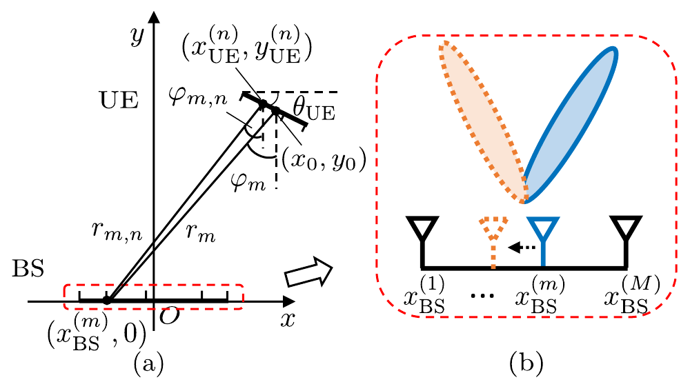
It is worth mentioning that we use a trigonometric transform to represent antenna positions. In the near field, directly using Cartesian coordinates would lead to complicated expressions, forcing us to introduce approximations with large errors. The trigonometric transform avoids this problem.

After some relatively mild approximations with lower error, we can approximate the distance as

Since the distance term in the near-field channel appears in the exponent, additive distances can be directly converted into multiplicative phases. We can use this to split the channel model into two parts:

where \({\bf D}_{\rm T}\) is a diagonal matrix that depends only on the distances $r_m$

while \({\bf P}\) contains only the cross terms related to the transmitter and receiver antenna positions. Handling matrix \({\bf P}\) is difficult because it contains the coupling relationships of all antenna positions. Therefore, we adopt a Taylor expansion¹

Analyzing the properties of the matrix, we find that matrix \({\bf P}\) can be truncated. At this point, the Taylor expansion result of this matrix can be written as a product of Vandermonde matrices

where

After simple transformations, it is easy to see that the problem of maximizing spectral efficiency can be approximately transformed into maximizing the determinant of a Vandermonde matrix (for details, see the journal version²). We rewrite the problem as follows:

The first term on the right-hand side is the equivalent form of the Vandermonde determinant, and the second term is the determinant form of the diagonal matrix, including a nonlinear transformation. The specific form of the external field is

Since $s$ is a variable in the angular domain, the optimal antenna position problem is thus transformed into a weighted Fekete-point problem in the angular domain. Due to the special form of the external field function, the closed-form solution is difficult to obtain. Therefore, in the conference version, we choose to use a greedy algorithm to solve it. This algorithm simulates the generation process of the Leja sequence, gradually selecting optimal points to construct the antenna position set. The pseudocode of the algorithm is as follows, with an additional simple position constraint to prevent antennas from being too concentrated.

Simulation results are shown in the figures below.

Achievable Rate Gain

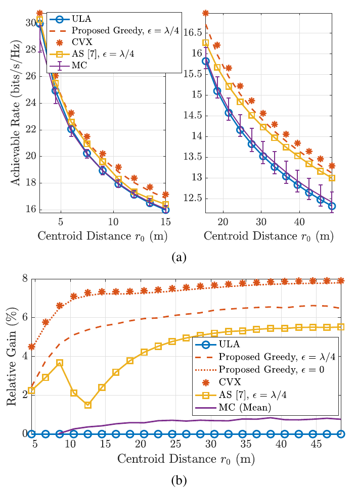
It is worth mentioning that under this nonlinear transformation, the original problem is actually convex, so we can also use CVX to solve it and compare the solution accuracy. The results are as follows.

Deviation Between Greedy and CVX Solutions

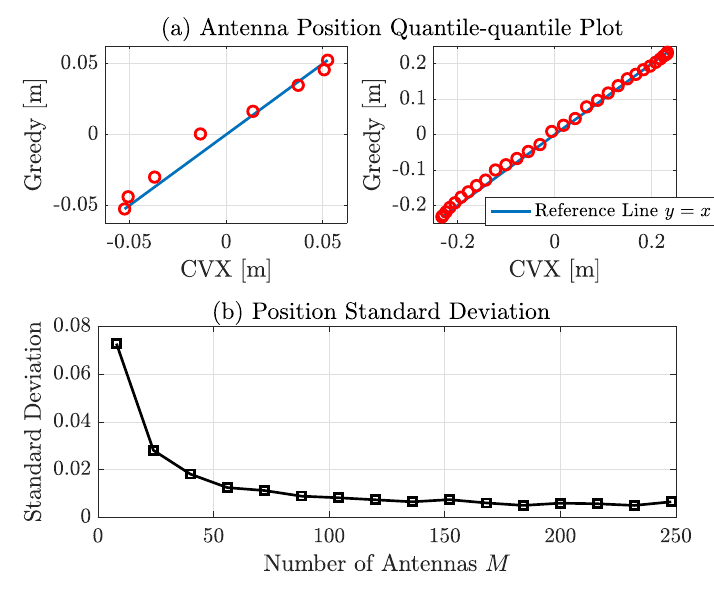
So, is there a way to obtain an exact analytical solution? The answer is yes. Taking the first-order equilibrium condition of the optimization objective, we get

Performing a first-order Taylor expansion on the external field term³, the original problem is transformed into

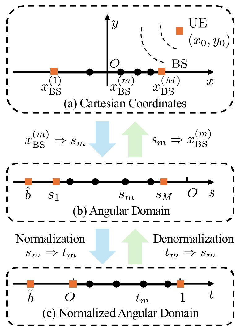
This equation is a charge equilibrium equation with interaction force \(1/\Delta r\) (traditional Coulomb force is inversely proportional to the square of the distance). The meanings of the related parameters are not elaborated here. Considering the normalization \(t = \frac{s-s_{\rm min}}{s_{\rm max}-s_{\rm min}}\in (0,1)\), the original charge equilibrium problem is transformed into the interval \((0,1)\)

The transformation process is shown in the figure below. We first transform the antenna positions into the angular domain \(s_m\), and then normalize them. By solving the normalized charge equilibrium problem and applying an appropriate inverse transformation to the results, we can obtain the optimal antenna positions.

Illustration of Charge Equilibrium Problem Transformation

To calculate the solution of the above equilibrium equation with sufficient efficiency and accuracy, it is very helpful to leverage some well-developed numerical algorithms. Here, we first assume that the optimal solution of the equilibrium equation is the root of a polynomial \(p(t)\), i.e.,

Then, using an existing result

the original equilibrium equation can be written as a second-order differential equation

where

This equation is known as the Heun equation, a very classical second-order linear differential equation, and there are many existing results on its properties⁴. One of the most important conclusions is that we can construct a tridiagonal matrix whose eigenvalues and eigenvectors can respectively give the corresponding normalized polynomial roots and polynomial coefficients. The proof of this part is more complex; see the original paper for details.

The complexity of the above solution method is still around \(O(M^3)\). However, since EVD methods have many software and hardware optimizations, the overall complexity is acceptable. For scenarios with very limited computing power, we further derive a closed-form approximate solution. First, since the external field function of the original problem is extremely weak, it is negligible under the influence of many internal charges (antennas). Therefore, we first ignore the external field, and the optimal solution of the equilibrium equation becomes the zeros of the \(M-2\)-order Jacobi polynomial \(P^{(1,1)}_{M-2}(t)\).

Considering that \(M\) is large, we can further approximate using the Jacobi recurrence relation to show that the original result weakly converges to the zeros of the Chebyshev polynomial \(P_{M-2}^{(-0.5,-0.5)}(t)\). At this point, the antenna positions can be approximately solved by the following closed-form expression

Through an appropriate linear inverse transformation, we finally obtain the optimal antenna positions under the massive MIMO asymptotic regime.

We also built a demo using Gemini-2.5-Pro, which can be experienced online via this link.

Citation

ICC’26:

@INPROCEEDINGS{icc26,
	author={Liu, Shicong and Yu, Xianghao},
	booktitle={IEEE Int. Conf. Commun. (ICC)}, 
	title={Near-Field Line-of-Sight Communication with Massive Movable Antennas}, 
	address={Glasgow, United Kingdom},
	year={2026},
	month={May},
	volume={},
	number={},
}

S. Liu, X. Yu, "Near-Field Line-of-Sight Communication with Massive Movable Antennas," {\em IEEE Int. Conf. Commun. (ICC)}, Glasgow, United Kingdom, May 2026.

Journal Version:

@ARTICLE{liu2026nf_ma,
	title={Near-Field Communication with Movable Antennas: An Electrostatic Equilibrium Perspective}, 
	author={Shicong Liu and Xianghao Yu and Shenghui Song and Khaled B. Letaief},
	year={2026},
  	volume={25},
  	number={},
  	pages={1-14},
	doi={10.1109/TWC.2026.3686424},
	note={Early Access},
}

S. Liu, X. Yu, S. Song, and K. B. Letaief, ``Near-Field Communication with Massive Movable Antennas: An Electrostatic Equilibrium Perspective'', IEEE Trans. Wireless Commun., 2026. Early Access.

Further Reading