TWC’25: 泛函分析最佳天线密度分布
TWC’25: Optimal Antenna Density via Functional Analysis

22 minutes read

Published: January 02, 2026

First of all, I would like to thank the reviewers and editors for their valuable comments, and for not rejecting the manuscript in the first round. The paper is currently under Major Revision; the arXiv preprint is already available. The second-round review is taking a bit long and no decision has been reached yet. Since the New Year holiday left me with some free time, I wrote these supplementary notes in case anyone is actually interested. If the manuscript is eventually accepted, I may add further comments here.

Because the research topic is, in my opinion, quite interesting and uses some less common mathematical tools, I would like to record some thoughts that arose during the writing process.

Motivation

Prof. K.-K. Wong has been promoting the concept of fluid antenna in the global communications community for a long time. Around 2021, when I was still a master’s student, Prof. Wong was invited to give a related seminar in Prof. Zhen Gao’s group at Beijing Institute of Technology. The introduction at that time still used the classic Bruce Lee line; in my impression, the lecture focused more on theoretical analysis and proof. Since I am not an antenna specialist, I did not pay too much attention to this direction at the time; I just felt it was very fancy.

Later, with the emergence of the movable concept, I gradually realized that changing antenna positions can have a non-negligible impact on communication performance. However, early research still focused on optimizing the positions of only a few antennas, because the algorithms proposed at that time suffered from sharply expanding solution spaces, high-polynomial optimization complexity, nonlinear constraints, and other issues as the number of antennas increased.

Since I was introduced to massive MIMO when entering the field (path dependence, one might say), my first instinct was still to consider scenarios with many antennas. But since conventional optimization algorithms are not easy to apply, I had to try a different approach.

For scenarios with many antennas, I first considered the spatial autocorrelation function as before¹:

$$ {\bf K}_f[n,n^\prime]= \frac{1}{M} \sum_{m=1}^{M} h\left({\bf r}_{\rm R}^{(n)},{\bf r}_{\rm T}^{(m)}\right)h^*\!\left({\bf r}_{\rm R}^{(n^\prime)},{\bf r}_{\rm T}^{(m)}\right). \label{eq:gram1} $$

Because we assume that the number of antennas is sufficiently large, this sum can be represented as a Riemann integral:

$$ \tilde{\bf K}_f[n,n^\prime] = \int_{1}^{M} h\left({\bf r}_{\rm R}^{(n)},{\bf r}_{\rm T}^{(m)}\right)h^*\left({\bf r}_{\rm R}^{(n^\prime)},{\bf r}_{\rm T}^{(m)}\right)\,{\rm d}m.\label{eq:gram2} $$

If we assume that each antenna position can be described by a function of the index $m$, i.e., $p = f(m)$, where $f(m)$ is strictly monotonically increasing, then via $m=f^{-1}(p)$ we obtain

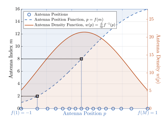
$$ \begin{align} \tilde{\bf K}_f[n,n^\prime] ={}&\int_{-1}^{1} h\left({\bf r}_{\rm R}^{(n)},\tilde{\bf r}_{ {\rm T} }^{(p)}\right) h^*\left({\bf r}_{\rm R}^{(n^\prime)},\tilde{\bf r}_{ {\rm T} }^{(p)}\right)\frac{\rm d}{ {\rm d} p} {f}^{-1}(p)\,{\rm d}p\notag\\ ={}&\int_{-1}^{1} w(p)h\left({\bf r}_{\rm R}^{(n)},\tilde{\bf r}_{ {\rm T} }^{(p)} \right) h^*\left({\bf r}_{\rm R}^{(n^\prime)},\tilde{\bf r}_{ {\rm T} }^{(p)} \right)\,{\rm d}p\notag\\ \triangleq{}&\tilde{\bf K}_w[n,n^\prime],\label{eq:kernel_p} \end{align} $$

where $w(p) = \frac{\rm d}{ {\rm d} p} {f}^{-1}(p)$ represents the number of antennas per unit length and is therefore the density function of the antenna positions.

Antenna positions and the corresponding density function

Computing the Optimal Density

Through the above process, it is natural to think that if we can find the optimal density function, we can also maximize the spectral efficiency. To obtain an optimal function, we need to use functional-analysis tools. However, direct functional analysis is still too complex for this problem, so we mainly adopt two approaches.

Numerical Optimization

Briefly, we treat the function as a vector on a grid of $P$ points, where the number of grid points is larger than the number of antennas, i.e., $P>M$. By computing the gradient, we construct a gradient-projection optimization algorithm. In the near-field scenario, we obtain the following density estimate:

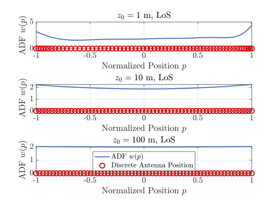
Density function from numerical optimization

It can be seen that the optimal density function has obvious peaks at the edges, which is consistent with the conclusion obtained later through the Szegő theorem.

(Extended) Szegő Theorem Analysis

Because the spatial autocorrelation matrix, called the Gram matrix in this paper, is essentially a Toeplitz matrix, we can use the Szegő theorem to asymptotically analyze its eigen-spectrum when the number of antennas is sufficiently large.

Under some reasonable near-field modeling, we can express the row/column entries of the Gram matrix as a truncated Fourier transform of the antenna density function:

$$ \begin{align} \overline{\bf K}_{f}\left[n,n^\prime\right] &=\frac{1}{z_0^2}\int_{1}^{M} \frac{e^{-\jmath\beta {\Delta n} p} }{\left( 1+ \tau p \right)^2 }\,{\rm d} f^{-1}(p)\label{eq:nflos_kernel}\\ &=\frac{1}{z_0^2}\int_{-1}^{1} \frac{w(p)}{\left( 1+ \tau p \right)^2} e^{-\jmath\beta {\Delta n} p }\,{\rm d} p\triangleq \overline{\bf K}_w\left[n,n^\prime\right]. \end{align} $$

where

$$ \begin{equation} \tilde{w}(p) = \frac{w(p)}{\left( 1+ \tau p \right)^2}, \end{equation} $$

is the weighted antenna density function. This function is also the generating function (symbol) of this Toeplitz matrix, and its properties determine the eigen-spectrum of the Gram matrix. In short, we have the following theorem:

Theorem 1 (Fisher-Hartwig Conjecture)²: For a real-valued generating function $s(\theta)$ defined on the unit circle, if it has $R$ singular points $\theta_r$ and takes the form:
$$ s(\theta)= b(\theta)\prod_{r=1}^{R} \left|2-2\cos\left(\theta-\theta_r \right) \right|^{\alpha_r}, $$
where $b(\theta)$ is a strictly positive and smooth function and $\alpha_r > -\frac{1}{2}$. The Toeplitz matrix $\bf T$ generated by this function satisfies the following asymptotic property:
$$ \begin{align} &\lim_{N\to \infty} \log \det \left( {\bf T}_N \right)\\ ={}& E_b\left(\theta\right) + \log N\sum_{r=1}^{R} \alpha_r^2 +\sum_{r=1}^{R} \frac{ {\rm BG}^2(1+\alpha_r)}{ {\rm BG}(1+2\alpha_r)}\\ &+\sum_{1\leq r<s\leq R} \left\vert2-2\cos\left(\theta_r-\theta_s \right) \right\vert^{-\alpha_r\alpha_s} + {\mathcal O}(1), \end{align} $$
where
$$ \begin{equation} E_b\left(\theta\right) =\frac{N}{2\pi} \int_{-\pi}^{\pi}\log b(\theta)\,{\rm d}\theta + E_0, \label{eq:eb} \end{equation} $$
$$ \begin{equation} E_0 = \sum_{k=1}^{\infty} k \left( \log b(\theta) \right)_k \left( \log b(\theta) \right)_{-k}<\infty, \label{eq:condszego} \end{equation} $$
and ${\rm BG}(\cdot)$ is the Barnes-G function, and $\left(\log b(\theta) \right)_k$ are the Fourier coefficients of $b(\theta)$.

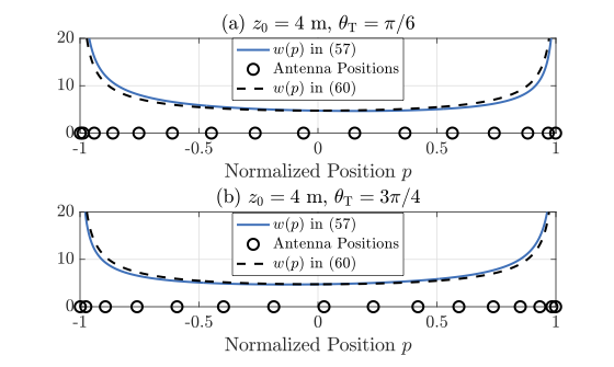
From the perspective of physical feasibility, we believe that singularities should exist only at the edges, and the higher the singularity, the stronger the spectral-efficiency gain (see the paper for details). For the case $\alpha = 0$, the optimal density function is

$$ \begin{equation} w(p;\alpha=0) \triangleq \frac{3\left( M-1 \right)}{6+2\tau^2} \left( 1+\tau p \right)^2. \end{equation} $$

For the case $-1/2<\alpha < 0$, the optimal density function is

$$ \begin{equation} w(p;-0.5\!<\!\alpha\!<\!0) \triangleq \left( \frac{\gamma_\alpha}{\left( 1 - p^2 \right)^{-2\alpha}} \!-\! \frac{\beta z_0^2}{2\pi\rho} \right) (1+\tau p)^2, \label{eq:optadf} \end{equation} $$

where $\gamma_\alpha$ is a normalization coefficient.

From Density Function to Discrete Antenna Positions

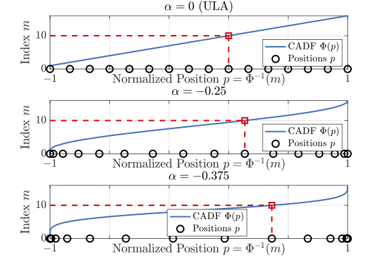
Since discrete antennas must ultimately be deployed, we need to convert the density function into concrete antenna positions. This paper adopts a simple inverse-cumulative-distribution-function method:

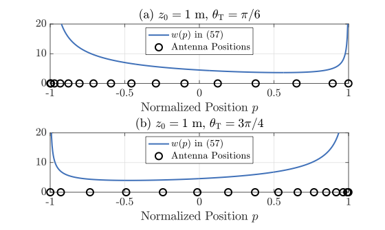
$$ \begin{equation} \Phi\left( p \right) = \int_{-1}^{p} {w}(p)\,{\rm d}p. \label{eq:cadf} \end{equation} $$

$$ \begin{equation} p = f(m) = \Phi^{-1}(m). \label{eq:cdfmethod0} \end{equation} $$

For massive MIMO and distances that are not extremely short, we also have a closed-form solution:

$$ \begin{equation} \begin{aligned} p &= \Phi^{-1}(m) = f(m)\\ &=\sqrt{B^{-1}\left(\frac{2m-\left(M+1\right)}{\gamma_\alpha};\frac{1}{2},1+2\alpha\right)}, \end{aligned} \label{eq:cdfmethod} \end{equation} $$

where $B^{-1}(\cdot)$ is the inverse incomplete beta function. It is worth noting that this is a very common and intuitive discretization method, and it is also very conducive to asymptotic analysis. When quantizing with this method, without additional physical constraints (e.g., antenna spacing limits), we can prove that as the number of antennas tends to infinity, the performance of the discrete antenna-position deployment scheme converges to the theoretical optimal density function.

Below are some density-function results:

Density functions and discrete antenna positions for different values of $\alpha$

Optimal densities and positions for different user locations

Citation Format

If you find this work helpful for your research, please consider citing:

@ARTICLE{11466358,
  author={Liu, Shicong and Yu, Xianghao and Xu, Jie and Zhang, Rui},
  journal={IEEE Trans. Wireless Commun.}, 
  title={Near-Field Communication With Massive Movable Antennas: A Functional Perspective}, 
  year={2026},
  volume={25},
  number={},
  pages={14455-14470},
  doi={10.1109/TWC.2026.3677546}}

S. Liu, X. Yu, J. Xu and R. Zhang, "Near-Field Communication With Massive Movable Antennas: A Functional Perspective," IEEE Trans. Wireless Commun. vol. 25, pp. 14455-14470, 2026.

If you are interested, please also stay tuned for our follow-up work.

~~To Be Continued~~

Shicong LIU