Our paper on near-field channel estimation based on discrete prolate spheroidal sequences (DPSS) has been accepted by the Wireless Communications Symposium of ICC’24. The pre-print is available on arXiv. This post briefly explains the proposed scheme and addresses a few reviewer concerns.
Background
Driven by extremely large-scale arrays such as RIS, wireless communications research is moving closer to optics: spherical-wave assumptions and diffraction effects are now routinely considered. In the near field, even a line-of-sight channel can support multiple streams because the channel matrix has higher rank. However, this also means that conventional compressed-sensing channel estimation requires more pilot overhead.
Many sparse-dictionary designs have been proposed, including polar codebooks, chirp codebooks, hierarchical codebooks, and even learned codebooks tailored to specific scenarios. These approaches have their own drawbacks: polar and chirp codebooks may lead to large dictionary sizes and non-orthogonal atoms, while learned codebooks incur high computational cost. We aim at a low-complexity dictionary with orthogonal atoms and good performance.
System Model
Consider a near-field user array communicating with a base station. The electric field at the receiver can be written via the Green’s function and the base-station current source:
\begin{equation} {\bf E}({\bf r}_{\rm R}) = \int_{ {\mathcal{S}_{\rm T} } } {\mathbf{G} }\left({\bf r}_{\rm T},{\bf r}_{\rm R}\right) {\bf J}({\bf r}_{\rm T})~{\rm d}{\bf r}_{\rm T}, \end{equation}
where the Green’s function is
\begin{align} {\mathbf{G}}\left({\bf r}_{\rm T},{\bf r}_{\rm R}\right) = {} & {} \frac{j\kappa Z_0 e^{j\kappa \Vert {\bf r} \Vert}}{4\pi \Vert {\bf r} \Vert}\left[ \left( {\bf I}-\hat{\bf r}\hat{\bf r}^H \right)+ \frac{j}{\kappa\Vert {\bf r} \Vert}\left( {\bf I}-3\hat{\bf r}\hat{\bf r}^H \right)\right.\notag\\ {} & {} \left. -\frac{1}{(\kappa \Vert {\bf r} \Vert)^2}\left( {\bf I}-3\hat{\bf r}\hat{\bf r}^H \right) \right]\label{green}\\ \simeq {} & {} \varphi_0 \frac{e^{-j\kappa \Vert {\bf r}\Vert}}{\Vert{\bf r}\Vert} \left( {\bf I}-\hat{\bf r}\hat{\bf r}^H \right).\notag \end{align}
The high-order terms are negligible outside the reactive near-field region, giving the commonly used spherical-wave model. Considering one polarization, the array response becomes
\begin{equation} {g}({\bf r}_{\rm T},{\bf r}_{\rm R}) = \varphi_0 \frac{e^{-j\kappa \Vert{\bf r}\Vert}}{\Vert{\bf r}\Vert}. \label{eq:sv} \end{equation}
For uniform linear arrays (ULA) on both sides, the LoS channel can be modeled as
\begin{equation} \begin{aligned} \mathbf{H}_{\rm LoS}[:,m] &= {\mathbf g}_{\rm R}({\bf r}_{\rm T}^{(m)})\\&= \left[ \tilde{g}({\bf r}_{\rm T}^{(m)},{\bf r}_{\rm R}^{(1)}),\cdots,\tilde{g}({\bf r}_{\rm T}^{(m)},{\bf r}_{\rm R}^{(N_{\rm R})}) \right]^{T}, \end{aligned} \label{eq:LoS} \end{equation}
where we define \(\tilde{g}(\cdot) = g(\cdot)/\varphi_0\) to absorb the constant \(\varphi_0\). For a simple Rician channel,
\begin{equation} {\bf H} = \sqrt{\frac{K}{1+K}}\mathbf{H}_{\rm LoS} + \sqrt{\frac{1}{1+K}}\mathbf{H}_{\rm NLoS}, \label{eq:channelmodel} \end{equation}
For convenience, define
\begin{equation} \begin{aligned} {\bf W}^{(t)} &= ({\bf W}_{\rm RF}^{(t)}{\bf W}_{\rm BB}^{(t)})^H\\ {\bf f}^{(t)} &= {\bf F}_{\rm RF}^{(t)}{\bf F}_{\rm BB}^{(t)}{\bf s}^{(t)} \end{aligned} \end{equation}
The single-shot observation model is
\begin{equation} {\bf y}^{(t)} = \left( ({\bf f}^{(t)})^{T}\otimes {\bf W}^{(t)} \right){\rm vec}({\bf H})+\tilde{\bf n}^{(t)} \end{equation}
Stacking multiple observations yields
\begin{equation} {\bf y} = {\boldsymbol{\Phi}{\bf h}}+\tilde{\bf n}, \label{eq:linearproblem} \end{equation}
The channel estimation problem can then be cast as a sparse recovery problem:
\begin{equation} \begin{aligned} {\rm(P1)}\quad\quad\underset{\tilde{\bf h}}{\min}\ &\ \Vert \tilde{\bf h} \Vert_0\\ {\rm s.t.}\ &\ \Vert\boldsymbol{\Phi} \boldsymbol{\Psi} \tilde{\bf h}-\mathbf{y}\Vert_2 \leq \varepsilon, \end{aligned} \end{equation}
This can be solved by convex relaxation, greedy iteration, or Bayesian inference. Greedy methods are attractive for their complexity/performance trade-off and are usually implemented as dictionary matching. The key question is therefore how to design a good near-field dictionary.
Proposed Scheme
We start from the transmit correlation matrix:
\begin{equation} \begin{aligned} {\bf R}_{\rm T} & \overset{~~~}{=} \mathbb{E}\left[{\bf H}^{H} {\bf H}\right]\\ & \overset{~~~}{=} \frac{K}{1+K}{\bf H}_{\rm LoS}^{H}{\bf H}_{\rm LoS}+\frac{1}{1+K}\mathbb{E}\left[ {\bf H}_{\rm NLoS}^{H}{\bf H}_{\rm NLoS} \right]\\ &\overset{~~~}{=} \gamma K{\bf H}_{\rm LoS}^{H}{\bf H}_{\rm LoS}+\gamma{\bf I}, \end{aligned} \label{eq:autocorr} \end{equation}
whose entries are
\begin{equation} \begin{aligned} {\bf R}_{\rm T}[m^\prime,m] &= \gamma K{\mathbf g}_{\rm R}^H({\bf r}_{\rm T}^{(m)}){\mathbf g}_{\rm R}({\bf r}_{\rm T}^{(m)})+\gamma {1}_{m,m^\prime}\\&=\gamma {1}_{m,m^\prime}+\gamma K\sum_{n=1}^{N_{\rm R}}\frac{e^{-j\kappa \Vert{\bf r}_{\rm T}^{(m)}-{\bf r}_{\rm R}^{(n)}\Vert }}{\Vert{\bf r}_{\rm T}^{(m)}-{\bf r}_{\rm R}^{(n)}\Vert} \\ &\quad\times\frac{e^{j\kappa \Vert{\bf r}_{\rm T}^{(m^\prime)}-{\bf r}_{\rm R}^{(n)}\Vert}}{\Vert{\bf r}_{\rm T}^{(m^\prime)}-{\bf r}_{\rm R}^{(n)}\Vert}, \end{aligned} \label{eq:autocorr2} \end{equation}
After a small approximation,
\begin{align} {\bf R}_{\rm T}[m^\prime,m] \approx &~ \gamma {1}_{m,m^\prime}\notag\\&~ +\frac{\gamma K}{r_0^2}\sum_{n=1}^{N_{\rm R}}e^{-j\kappa\frac{\left(x_{\rm T}^{(m)}-x_{\rm R}^{(n)}\right)^2-\left(x_{\rm T}^{(m^\prime)}-x_{\rm R}^{(n)}\right)^2}{2y_0}}\notag\\ =&~\gamma {1}_{m,m^\prime}+\frac{\gamma K e^{j\kappa \frac{(x_{\rm T}^{(m^\prime)})^2-(x_{\rm T}^{(m)})^2}{2y_0}}}{r_0^2 } \label{eq:dft}\\ &~\times\sum_{n=1}^{N_{\rm R}} e^{j\kappa\frac{x_{\rm R}^{(n)}\left(x_{\rm T}^{(m)}-x_{\rm T}^{(m^\prime)}\right)}{y_0} }\notag\\ \triangleq&~\gamma {1}_{m,m^\prime}+\gamma K e^{j\kappa \frac{(x_{\rm T}^{(m^\prime)})^2-(x_{\rm T}^{(m)})^2}{2y_0}} {\bf R}^\prime_{\rm T}[m^\prime,m],\notag \end{align}
The EVD of this matrix satisfies
\begin{equation} {\bf R}_{\rm T}{\bf v}_m = {\bf D}_{\rm T}^{-1} \left( \gamma K\mathbf{R}^\prime_{\rm T}+\gamma {\bf I} \right){\bf D}_{\rm T}{\bf v}_m = \lambda_m{\bf v}_m, \label{eq:evd} \end{equation}
where the position-dependent phase term is pulled out as
\begin{equation} {\bf D}_{\rm T} = {\rm diag}(e^{j\kappa \frac{(x_{\rm T}^{(1)})^2}{2y_0}},\cdots,e^{j\kappa \frac{(x_{\rm T}^{(N_{\rm T})})^2}{2y_0}}). \label{eq:compensation} \end{equation}
It does not affect the eigenvectors. The remaining correlation matrix can be written as
\begin{equation} \begin{aligned} {\bf R}_{\rm T}^\prime[m^\prime,m] & \overset{~~~}{=} \frac{1}{r_0^2} \sum_{n=1}^{N_{\rm R}} e^{j\kappa\frac{x_{\rm R}^{(n)}\left(x_{\rm T}^{(m)}-x_{\rm T}^{(m^\prime)}\right)}{y_0} }\\ &\overset{(a)}{\approx} \frac{1}{r_0^2} \int_{-L_{\rm R}/2}^{L_{\rm R}/2}e^{\frac{j\kappa}{y_0}x (x_{\rm T}^{(m)}-x_{\rm T}^{(m^\prime)})} {\rm d}x \\ &\overset{~~~}{=}\frac{ 2y_0\sin\left[ \frac{\kappa L_{\rm R} (x_{\rm T}^{(m)}-x_{\rm T}^{(m^\prime)} )}{2y_0} \right] }{ r_0^2 \kappa \left(x_{\rm T}^{(m)}-x_{\rm T}^{(m^\prime)} \right)}\\ &\overset{~~~}{\propto}\frac{\sin\left[2\pi W (x_{\rm T}^{(m)}-x_{\rm T}^{(m^\prime)}) \right] }{ \left(x_{\rm T}^{(m)}-x_{\rm T}^{(m^\prime)} \right)}, \end{aligned} \label{eq:toeplitzmat} \end{equation}
which is exactly a sinc kernel. The corresponding eigenvectors form the DPSS dictionary, which is orthogonal and admits fast algorithms.
A summary of the dictionary design is shown below.
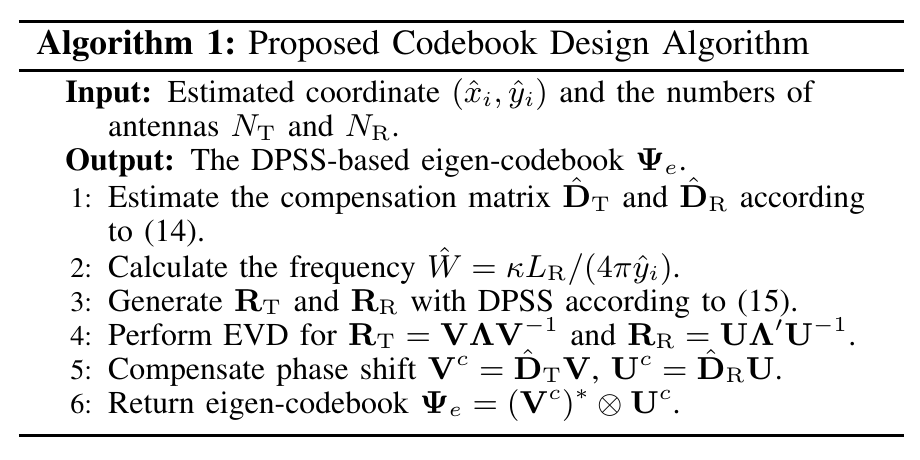
DPSS dictionary design flow
Simulation Results
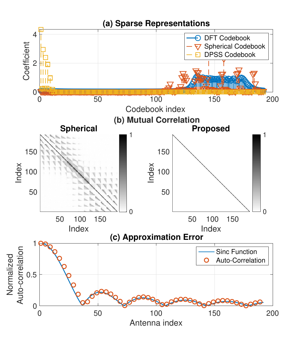
Codebook sparsification and orthogonality
The first result shows that the proposed codebook sparsifies the near-field channel well, yields nearly orthogonal atoms, and the approximation error is negligible compared with DFT and polar dictionaries.
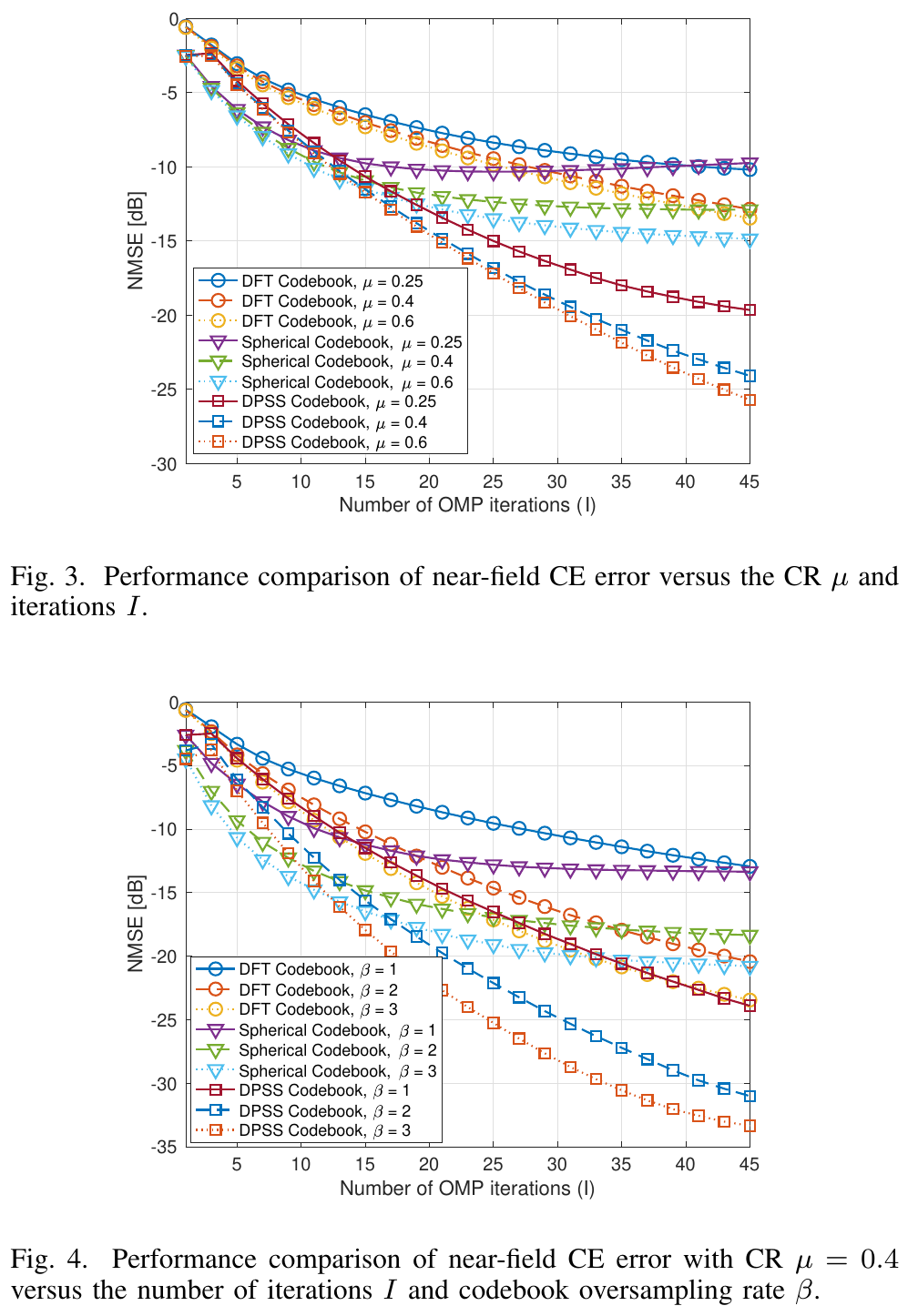
Performance under different measurements and redundancy
The next two figures compare performance under different numbers of measurements and dictionary redundancy. The DPSS codebook consistently outperforms the baselines.
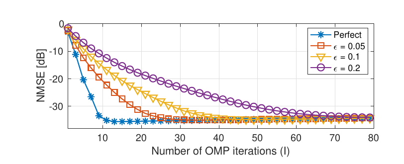
Estimation-error convergence across distances
The figure above shows the convergence of the estimation error across different distance ranges.
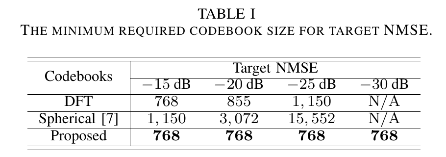
Dictionary size required for target performance
Finally, the table compares the dictionary sizes required to achieve a target performance.
Citation
@INPROCEEDINGS{10622872,
  author={Liu, Shicong and Yu, Xianghao and Gao, Zhen and Ng, Derrick Wing Kwan},
  booktitle={IEEE Int. Conf. Commun. (ICC)},
  title={DPSS-Based Codebook Design for Near-Field XL-MIMO Channel Estimation},
  address={Denver, CO, USA},
  year={2024},
  pages={3633-3638},
  doi={10.1109/ICC51166.2024.10622872}}
S. Liu, X. Yu, Z. Gao and D. W. K. Ng, "DPSS-Based Codebook Design for Near-Field XL-MIMO Channel Estimation," in Proc. IEEE Int. Conf. Commun. (ICC), Denver, CO, USA, Jun. 2024, pp. 3633-3638.